
Last year, we rebuilt our cost-based optimizer from scratch for CockroachDB’s 2.1 release. We’ve been continuing to improve the optimizer since then, and we’ve added a number of new features for the CockroachDB 19.1 release. One of the new features is automatic collection of table statistics. Automatic statistics enables the optimizer to make better decisions when choosing query plans.
This post explains why statistics are important for the optimizer and describes some of the challenges we overcame when implementing automatic collection.
A Tale of Two Queries
Consider the following two SQL queries, used by an imaginary kitchen supplies company to count the number of toaster ovens purchased by customers in New York City, grouped by the date of purchase:
SELECT count(*), o.purchased
    FROM products AS p,
         orders AS o,
         customers AS c
    WHERE c.id = o.cust_id
         AND p.id = o.prod_id
         AND c.city = 'New York'
         AND p.type = 'toaster oven'
GROUP BY o.purchased;
Query A
SELECT count(*), o.purchased
    FROM customers AS c,
         orders AS o,
         products AS p
    WHERE c.id = o.cust_id
         AND p.id = o.prod_id
         AND c.city = 'New York'
         AND p.type = 'toaster oven'
GROUP BY o.purchased;
Query B
With minimal optimization, these queries correspond to the following logical query plans:
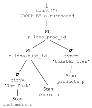
Query A

Query B
These queries compute the same result, but one query is vastly more expensive than the other. Can you tell which one? (scroll down to see the answer…)
.
.
.
.
.
.
.
.
.
Spoiler alert: it’s not possible to determine which query is faster without more information. So suppose I give you the following statistics:
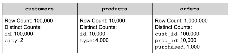
Table 1
Now can you tell?
Before I give the answer, let’s discuss what makes a query expensive in the first place, and why you should care. The “cost” of a query roughly translates to the total amount of computing resources required to execute the query plan, including CPU, I/O and network. Lower-cost plans tend to execute faster (i.e., they have lower latency), and also enable the system to maintain a higher throughput, since more resources are available for executing other queries simultaneously. That means less money spent on extra hardware, and less time waiting for results!
How do you estimate the cost of a query?
We can estimate the cost of a particular query plan by estimating the cost of each operation in the plan and adding them together. For example, consider Query Plan A. You can think of data as flowing through the plan from bottom to top. First we scan table customers and apply a filter, then we scan table orders and join the two together, etc. Each stage in the plan costs a certain amount depending on the type of operation and the amount of data that must be processed. Operations involving I/O are generally more expensive than operations involving only CPU, so reading 10,000 rows from disk (e.g., as part of a scan) is much more expensive than applying a filter to those rows. The actual cost formula varies for each operator and is beyond the scope of this blog entry, but the important thing to know is that the cost of each operation is directly proportional to the number of rows processed.
So how do we estimate the number of rows processed by each operator? With statistics, of course!
Similar to how data propagates from the bottom to the top of a query plan, we can also propagate statistics from the bottom to the top to estimate the number of rows at each step.
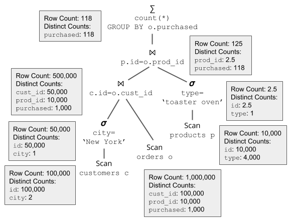
Query Plan A with Statistics
Let’s look at the example of query plan A. Given the stats from Table 1, we know that customers has 100,000 rows. Since in this simple example we don’t have any indexes on customers, the scan must process all of the rows. Similarly, the filter operator must process all rows produced by the scan to test the filter predicate city='New York' on each row. But this is where it gets interesting. To estimate the number of rows that match the filter predicate and pass on to the join operator, we need to calculate the selectivity of the filter, or the percentage of rows that are likely to match. For this calculation, we make the simplifying assumption that all values are uniformly distributed in each column. For example, we assume that a column with 30 rows and 3 distinct values will have 10 of each value.
In our running example, we can see from Table 1 that column city has only two distinct values (it turns out our imaginary kitchen supply company only has two locations). After we apply the predicate city='New York', there is at most one distinct value, the value 'New York'. Utilizing the assumption of uniformity, we can estimate the selectivity of the predicate as 1⁄2. With 100,000 input rows, we estimate that after the predicate is applied there will be 100,000 * 1⁄2 = 50,000 rows.
Note that this result of 50,000 rows is just an estimate, since the assumption of uniformity is not always correct. It’s possible that the data is skewed and nearly all of all rows match city='New York'. It’s also possible that almost none of the rows match city='New York'. In the next release we will incorporate histograms into our estimates to handle such cases. But in practice, the uniformity assumption works reasonably well for query optimization.
The cost-based optimizer does not need to know the exact cost of a query plan; it just needs a good enough estimate that it can compare two plans and select the relatively cheaper plan.
Given that we estimate 50,000 rows from the filter, how do we propagate the statistics up the tree? We can’t directly apply the 0.5 filter selectivity to the distinct count, since that would be statistically incorrect. Suppose that there is another column in customers that tracks the customer’s gender. Assuming that gender is independent of city (which is true, last time I checked…), it is likely that gender will still have (at least) two distinct values after half of the rows are removed that don’t match city='New York'. If we were to blindly apply the selectivity to distinct counts (similar to how we applied it to the row count), we would estimate that gender had only one distinct value, which is clearly incorrect given the assumption of independence. Instead, we use the following formula:
d′=d−d∗(1−selectivity)n/d
Where n is the number of input rows, d is the distinct count before the selectivity is applied, and d ’ is the distinct count after. It can be derived as follows: If each distinct value appears n/d times, and the probability of a row being filtered out is (1−selectivity), the probability that all n/d rows are filtered out is (1−selectivity)n/d. So the expected number of values that are filtered out is d∗(1−selectivity)n/d. This formula has the nice property that it returns d∗selectivity when d=n but it’s closer to d when d<<n.
Similar to the uniformity assumption, the independence assumption is not always correct, but it makes calculations significantly simpler. We’ll likely relax the independence assumption in future releases of the optimizer.
Moving further up the query plan, we must next calculate the number of rows produced by the join. This is a notoriously difficult problem, and remains an open area of research1. For equi-joins such as the ones in queries A and B, we make the simplifying assumption that we have a primary key-foreign key join, so the output cardinality will be equal to the larger of the two inputs multiplied by the selectivity of any filters that have been applied. Distinct counts are not affected significantly by joins.
As the last step in both query plans, we apply a GROUP BY operation which calculates the number of matching orders grouped by purchased date. Luckily, calculating the number of output rows of a GROUP BY operator is easy: it’s equal to the number of distinct values of the grouping column(s).
Although this example only covers a subset of all SQL operators, it gives a good flavor for how we use statistics to estimate the cost of different query plans. Hopefully now you can see that query A is significantly more expensive than query B. The CockroachDB optimizer will always transform query A so that it uses the same query plan as B. And for good reason: when we execute the two plans, we see that query A takes 1.9 seconds while query B takes 16 ms: over a 100X difference!
How CockroachDB Collects Table Statistics
So how do we get statistics such as the ones shown in Table 1 that are used by the optimizer to calculate the cost of candidate query plans? In CockroachDB, we collect statistics using the command CREATE STATISTICS. CREATE STATISTICS performs a distributed, full table scan of the specified table, and calculates statistics in parallel on each node before a final merge (see Figure 1). After collection, statistics are stored in the system table system.table_statistics, and are cached on each node for fast access by the optimizer.
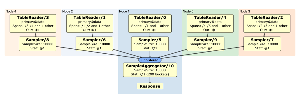
Figure 1: The distributed SQL plan of a CREATE STATISTICS statement on 5 nodes
The statistics we currently support are:
Row Count
This is an exact row count as of the time of the table scan. Although this is the simplest statistic, it’s also the most important. As you learned in the previous section, row count is the primary input to our cost model for determining the cost of each candidate query plan.
Distinct Count
For each index column and a subset of other columns in each table, we estimate the number of distinct values. As described above, distinct counts are useful for estimating the selectivity of filter predicates and estimating the number of rows output by GROUP BY and other relational SQL operators. We don’t calculate exact distinct counts, because for columns with many distinct values, the calculation could require nearly as much memory and disk space as the entire table itself! Instead, we use a variant of the well-known HyperLogLog algorithm called HLL-TailCut+2 and the excellent golang implementation by Axiom, Inc3. HyperLogLog estimates distinct counts with high accuracy and very low memory overhead. It can also be calculated in parallel across several nodes and efficiently merged to produce a distinct count estimate for the full table.
Null Count
We calculate null counts explicitly, as NULL is a value that can appear quite often in some workloads. We can get better cardinality estimates for certain queries by tracking this count separately.
In the future, we plan to support more statistics, including multi-column distinct counts and histograms.
Changes to Table Statistics in CockroachDB 19.1
The CREATE STATISTICS command existed in the 2.1 release, but we found that most customers were not taking advantage of it, and the few that knew about it were not using it effectively. There were a few reasons for this:
We did not advertise the feature, so many customers were not aware of it. We did this purposefully, since as described below,
CREATE STATISTICSis difficult to use correctly.Even if they discovered the command on their own, they might have run it once and forgotten to run it again. This is a problem because statistics can quickly become stale for tables that are modified frequently. Running
CREATE STATISTICSonce can be worse than never running it at all, since we have some reasonable defaults in the optimizer if there are no stats. But we’ll always use whatever stats are available, so suppose you create a table, add one row, and then runCREATE STATISTICS. And then you add 1 million rows but forget to refresh the stats. The optimizer will choose a plan optimized for the case of one row, even though that may be an awful plan for the case of one million rows.A savvy user might have realized that they needed to refresh stats periodically, but then it was not clear how often to perform a refresh.The optimal frequency may be different for every table, since some tables are updated frequently and others are updated less frequently. Furthermore, some tables are large, and even a lot of updates don’t change the stats much, while some tables are small and a few updates can drastically change the stats.
Even if a user managed to overcome all of these hurdles, we were not satisfied with the status quo. Our mission at Cockroach Labs is to “make data easy”, and forcing users to perform their own periodic stats refreshes did not fit with this mission.
The Solution: Automatic Statistics Collection
The solution, of course, is for CockroachDB to perform statistics collection automatically. Our idea at the beginning of the release was to detect when some significant portion of the data in a table had changed, and then automatically trigger statistics collection by having the system call CREATE STATISTICS. This introduced two key challenges:
We want to detect when a significant amount of data has changed, but there should be negligible impact on the performance of
INSERT,UPDATEandDELETEtransactions.Once we’ve decided to trigger a statistics refresh, the collection of statistics should have negligible impact on the performance of concurrent transactions.
Let’s examine each of these challenges:
Deciding to Trigger a Refresh
In order to decide when to trigger a refresh, we want to know when a “significant” portion of a table has changed. To make this concrete, let’s say that we want to update stats after approximately 20% of the rows in a table have been inserted, updated or deleted. The advantage of using a percentage instead of an absolute row count is that it allows the frequency of refreshes to scale inversely with the size of the table.
So the challenge is to determine when 20% of rows have changed. Perhaps you’re thinking, “this doesn’t seem very hard…”. At first glance, it does seem straightforward; we know how many rows are affected by each mutation operation on each node. But the problem is that we can have many mutation operations happening simultaneously to the same table on different nodes, and we’d like to avoid having a central counter somewhere that could be a source of contention. The only way a geo-distributed system like CockroachDB scales is if nodes are largely independent.
Luckily, the decision to refresh a table after some percentage of rows have changed does not need to be exact. There is a tradeoff between more frequent refreshes (which add overhead to the cluster), and less frequent refreshes (which could result in suboptimal query plans). We have found that refreshing with 20% of rows “stale” provides a good balance, but 10% or 30% would also be perfectly fine in most cases.
Given this flexibility, we decided to solve the problem by using the following statistical approach: after every mutation operation (e.g., INSERT, UPDATE or DELETE), there is a small chance of statistics getting refreshed. In particular, the probability of a refresh is:
P(refresh) =
To implement this statistical approach, we essentially use the following simple algorithm (although there are some complexities discussed in the next section): after each mutation, generate a random number between 0 and 1, and if it falls below this probability value, kick off a CREATE STATISTICS run. What this means is that over time, stats for each table are refreshed after approximately 20% of rows have changed. We also have some guard rails in place in case there are statistical outliers. In particular, we always refresh stats for a table if it has no stats yet or if it has been a long time since the last refresh.
Running the Refresh
The second challenge was ensuring that running a statistics refresh did not significantly impact running workloads. It’s one thing if there is high overhead when a user knowingly runs CREATE STATISTICS on the command line, but it’s another thing if we trigger it without their knowledge and all of a sudden the command is using half the resources in the cluster. Since a statistics refresh can happen at any time, it must have minimal overhead.
This requirement forced us to rethink the solution described in the last section for triggering a refresh after 20% of rows changed. In particular, the simple algorithm of possibly triggering a refresh after each mutation was problematic. There can be many updates per second, but each CREATE STATISTICS run can take minutes. As a result, we could have multiple threads scanning the same table to collect statistics at the same time. This is a big problem, since a single full table scan can impact performance. Many table scans at once can actually bring down the cluster.
The solution we came up with was to have one background “refresher” thread running on each node. Mutation operations such as INSERT, UPDATE and DELETE send messages to that thread with the table and number of rows affected, and the refresher aggregates the counts of rows updated for each table on that node. Periodically, the refresher thread starts up a separate thread that uses the latest counts to possibly kick off a statistics refresh for each table.
The background refresher thread ensures that at most one statistics refresh is triggered at once per node, but it does not provide any coordination between nodes. To ensure that at most one automatic statistics refresh is running globally on the cluster, we took advantage of the existing “jobs” infrastructure used to run commands like IMPORT, BACKUP and RESTORE. In the last release, CREATE STATISTICS was a normal SQL statement, but we changed it during this release cycle to run as a job. Now, every time CREATE STATISTICS is called, it creates an entry in the system.jobs table. If a node wants to perform a refresh, it first checks the system.jobs table to be sure that there are no other statistics jobs currently running. In this way, we ensure that only one statistics refresh is active at once. The jobs infrastructure ensures that we always make progress, since if a node dies, another node will adopt the job.
Even with all of this infrastructure in place, we found that the overhead of a single CREATE STATISTICS job was too high for some workloads. Workloads with heavy utilization of resources saw throughput drops and latency spikes each time a statistics refresh started. This observation led us to the final requirement: we needed to limit the overhead of each individual CREATE STATISTICS job. The solution we used was to throttle the execution of statistics collection. Specifically, we insert some idle time (i.e., sleep) after every 10,000 rows are processed. The amount of idle time is adaptive, and depends on the current CPU utilization of the cluster. If utilization is high, we sleep more, and if utilization is low, we turn off throttling altogether.
The Practical Stuff
By this point you may be wondering, “How do I actually use this feature?” Consistent with our mission to “make data easy”, you don’t need to do anything other than upgrade to CockroachDB 19.1. Automatic statistics are enabled by default in 19.1, so unless you explicitly disable the feature, the system will trigger statistics refreshes as needed.
Although we’ve made every effort to minimize the impact of automatic statistics collection on performance of the system, there will always be overhead due to the cost of performing a full table scan for each refresh. For most workloads, the amortized impact on performance is less than 1%, but we’ve seen some cases with larger performance degradation. If your workload is negatively affected, our documentation on the automatic statistics in CockroachDB describes how you can adjust the frequency of refreshes or disable automatic collection altogether. It’s still possible to run CREATE STATISTICS manually if you want full control over when stats are refreshed.
Conclusion
We hope this post has convinced you that statistics are essential for the optimizer to produce good query plans for a wide variety of queries, and we hope it has allowed you to peek inside the optimizer to learn a bit about how it works. CockroachDB 19.1 provides tools to collect statistics both manually and automatically, with the goal of keeping statistics fresh for the optimizer to use with minimal performance impact.
Happy querying!
Notes
See, for example, A. Kipf, T. Kipf, B. Radke, V. Leis, P. A. Boncz, and A. Kemper. Learned cardinalities: Estimating correlated joins with deep learning. CoRR, abs/1809.00677, 2018 [return]
Q. Xiao, Y. Zhou and S. Chen, “Better with fewer bits: Improving the performance of cardinality estimation of large data streams,”
IEEE INFOCOM 2017 - IEEE Conference on Computer Communications, Atlanta, GA, 2017, pp. 1-9.[return]


