AWS Database Blog
Speed up time series data ingestion by partitioning tables on Amazon RDS for PostgreSQL
In the post Designing high-performance time series data tables on Amazon RDS for PostgreSQL, we explained how to use partitioned tables as a strategy to improve performance when handling time series data. In this post, we focus on data ingestion and why partitioned tables help with data ingestion.
PostgreSQL has had the ability to handle table partitioning for a while now. Before PostgreSQL 10, you could create partitions by using triggers and table inheritance, which allowed you to customize how your partitions work. However, this was complex and difficult to maintain. PostgreSQL 10 introduced declarative partitions. Declarative partitions (also known as native partitions) removed the hassle of defining check constraints, which made sure that the optimizer excludes unnecessary partitions during a table scan. This is also known as partition pruning. Declarative partitioning removes the need of placing triggers on the parent table to redirect writes to each partition.
Since PostgreSQL 10 was released in 2017, many improvements have been made and continue to be made by the PostgreSQL community. These improvements include a variety of features, such as performance improvements, better integration with other engine components such as foreign data wrappers, and support for logical replication.
The idea of partitioning is that the database engine performs better by having small chunks of data (objects or partitions) to process when compared to processing a single, large table. This is true not only when you need to read the table, but also when you ingest new rows of data. This post focuses on why partitioned tables help with data ingestion. If you haven’t read the first post, we strongly recommend you do so. It will help you better understand the context of this post.
Performance factors
Several factors affect the performance of the operation to insert (or ingest) rows in a table. It’s important to understand each of these factors to better tune your database to meet your needs. In this post, we discuss the following:
- Table size
- Indexes
- Ingestion method
- Checkpoints
- Availability Zones
Table size
We refer to table size as number of rows and space consumed in disk. When speaking strictly about data ingestion, the size of the table alone doesn’t have a significant impact on the performance ingestion. In most use cases, a large table must also be read. The larger the table, the slower the reads are. To help speed up reads, you create indexes, but there’s a catch—the more indexes a large table has, the slower the data ingestion.
Indexes
Related to table size, but with its own importance, is the number of indexes associated with a table (also their sizes, number of columns, and methods). An index impacts data ingestion performance because the index must always be ordered. By default, a PostgreSQL index uses a balanced tree data structure (or BTree for short) to store all values for the columns that are being indexed. Index values must be ordered and have a pointer to the table itself (which doesn’t necessarily have to store data in an ordered way). To keep the index ordered, the BTree algorithm has to split the data structure, keep the correct position, and maintain order so that index doesn’t end up having one branch larger than the other. This keeps a uniform speed when it’s read, and is also the reason why we strongly recommend not creating more indexes than you really need.
You can query your database to identify all indexes that aren’t used:
In the preceding example, we’re joining catalog tables (pg_index and pg_stat_indexes) that store index definitions, its schemas, and the number of times each index was used, which is determined by the column idx_scan. We filter out primary keys and unique indexes—even though they’re not being used, they serve a purpose in your schema definition.
Another important tuning is to remove duplicated indexes (two or more indexes with the same definition). For an example query to identify duplicate indexes, see Duplicate indexes.
Ingestion method
There is an important difference in performance when ingesting a large number of rows at one time (bulk insert through COPY command) vs. inserting multiple rows using INSERT, even when those inserts are in the same transaction. For example, using COPY to ingest one million rows is always faster than using one million insert statements. INSERT is slower because each time you issue the INSERT command, the PostgreSQL engine has to parse and check if the command grammar is correct. When COPY is used, it’s assumed that you already have the data you want to ingest upfront (you’re importing data). COPY is recommended for bulk load operations. This is important to understand because you may not always have the opportunity to use COPY. Most applications use INSERT to append or add rows in a table. The following are some examples where we correlate use cases with commonly used ingestion methods:
- IoT and DevOps – Applications used by IoT sensors and data collection agents insert data directly into the table, through the INSERT statement or through small batches using COPY. COPY is usually used during the backup to export or import data, but can also be called directly from many connections drivers such as JDBC, psycopg2, or DBD::Pg, for example.
- Historical dataset – For a complete dataset, you can use COPY or a common table expression (CTE). If you already have the dataset you’re ingesting in a CSV file, you can use COPY. If the historical data is being retrieved from another table (even from a remote table through a foreign data wrapper), then it’s possible to use a CTE where you INSERT data into the other, based on the result of a SELECT query.
Checkpoints
Every time a checkpoint operation occurs, a full-page write operation also occurs. This happens in order to ensure the 8 kB page (a database block in memory) is fully written into the file system (which has its smaller page defined as 4 kB). The full-page write is a technique that ensures your database doesn’t write a partial page in case of a failure, potently creating data corruption. All Amazon Relational Database Service (Amazon RDS) for PostgreSQL instances enforce full-page writes. Because we’re ingesting too much data in short periods, using tables that have many indexes, and due to the full-page writes, it’s highly likely that you’re checkpointing too often and also writing more than you need. If so, the following message appears in your database logs:
If you see this message, you should tune your checkpoint parameters.
Availability Zones
A factor that can’t be neglected when ingesting a large amount of data into a database is how far the database is from the source or application that is ingesting data. If your application or source is on a certain Availability Zone, for example, us-west-2d, then you want to have your RDS for PostgreSQL DB instance in the same Availability Zone to avoid network latencies between two different Availability Zones. Even though the latency difference appears minimal, when ingesting a large number of rows, this can have a significant performance impact using the INSERT method. Paying attention to Availability Zones is particularly important when benchmarking two instances with different settings or using different strategies. Make sure both instances are in the same Availability Zone to prevent skewed results due to network latency.
Data ingestion examples and benchmarks
You can choose from several tools to simulate large amounts of data ingestion. These tools allow you to ingest data as fast as possible so you can compare different approaches. For example, you can compare a bulk load type data ingestion while having a single table with multiple indexes and a partitioned table with those same indexes. You can also compare different parameter settings. However, we don’t recommend changing multiple variables at the same time, so you can understand exactly the performance benefit of each change. For example, if you’re comparing partitioned tables vs. a single table, don’t change other parameters (this way, you’ll have a fair comparison).
In this post, we show two different tools for benchmarking and comparing data ingestion: tsbs and pgbench. Many other tools exist (like HammerDB or Sysbench), each one having its own characteristics and specialties.
Ingestion examples: tsbs
In the post Designing high-performance time series data tables on Amazon RDS for PostgreSQL, we show a data ingestion example using tsbs, a simple but great benchmark tool designed to measure time series data across multiple databases. To ingest as quick as possible, tsbs requires you to generate the dataset you want to ingest in advance.
The tsbs tool simulates two use cases: DevOps and IoT. The DevOps use case simulates a system or host monitoring system. The IoT use case simulates tracking a fleet of trucks belonging to a fictional truck company, simulating environmental factors such as fuel level. For this post, we use the IoT use case.
By default, tsbs doesn’t pre-create native partitions, so in the following examples we handle native partitions by creating the tables ourselves using pg_partman to handle the creation of each partition automatically.
To compare data ingestion between partitioned and non-partitioned tables, we can install tsbs.
First, we install golang, a dependency for tsbs:
With golang successfully installed, we install the benchmark tool, tsbs:
If all these steps were successful and no failures occurred, you should see the following command returning 25 (meaning 25 lines were found, or 25 commands inside the $GOPATH/bin directory starting with the tsbs_ string).
Now, we generate data that we use in the tests. For that, we create a new directory and call the program tsbs_generate_data:
You must use the timescaledb format parameter to generate data, even when you’re generating data for PostgreSQL native partitions. When used in combination with iot, the scale parameter defines the total number of trucks tracked.
The preceding command generates 3 days of data, where the timestamp interval is preset between 2021-06-08 00h00m00s and 2021-06-10 23h59m59s. In our test host (a m5.16xlarge instance, deployed in the same Availability Zone) this command took 20 minutes, producing a compressed file of 3.1 GB.
After the dataset is generated, we’re ready to start our first data ingestion. For this post, we ingest data into an RDS for PostgreSQL DB instance running PostgreSQL 13.2. We start with an example without partitions or optimizations. The instance class used for this test was a db.r6g.4xlarge with 8 TB storage and 20,000 IOPS. Choose your preferred instance class, bearing in mind that different instances classes have not only different amounts of vCPUs and memory, but also different I/O throughput capabilities. For more information, Network Performance.
Ingest into single tables
To make things easier, we set PostgreSQL’s connection environment variables and use them when calling the load script:
The load script is inside the tsbs source code (which we downloaded using the git command earlier):
Note the parameters --workers=4 and --batch-size=10000 that we’re passing to the tsbs_load_timescaledb command. The first defines how many concurrent connections ingest data through the COPY command. Also, for each worker, a second connection is created to ingest rows into the tags table. The second parameter defines how many rows are ingested by each worker. Theoretically, with more workers, you can ingest more data at the same time; however, with more workers, your DB instance has to have more resources like CPU, memory, and I/O to handle the workload.
The parameter --use-hypertable=false tells the load command that we’re not using the timescaledb extension, which uses a different approach for partitioning.
The database ingested 186,706,431 rows from four workers (or concurrent sessions) using COPY as the ingestion method, with each worker batching 10,000 rows. These rows were inserted into two tables, diagnostics and readings, with sizes of 17 GB and 21 GB, respectively. None of those tables were partitioned, and the whole ingestion process took 1,784 seconds (approximately 29 minutes).
The data was pre-generated and the Amazon Elastic Compute Cloud (Amazon EC2) instance we used to ingest the data (meaning to run the tsbs program) was powerful enough to handle four parallel workers. Also, the RDS instance was deployed into the same Availability Zone where the EC2 instance running tsbs was deployed. The RDS instance was powerful enough that we can focus only on the differences between partitioned tables and using non-partitioned (normal or single) tables.
To analyze how many rows are being ingested over time, we save the ingestion report in the file $HOME/data_load_metrics_iot-single-table-Jun21_rpg13.log.
The following code shows these two table definitions and their sizes:
Below the total size of the database:
Ingest into partitioned tables
Now that we have ingested our rows using a single table (non-partitioned) approach, we do the same using partitioned tables. To achieve this, we create the objects used during the ingestion manually and use the pg_partman extension to automatically create the partitions. To learn more about partitioning in an Amazon RDS environment, see Managing PostgreSQL partitions with the pg_partman extension.
Before we connect, we define the connection variables to be used during object creation and the benchmark:
We can now create the objects through the psql client:
After we create the objects, we can start the benchmark ingestion by using the tsbs_load_timescaledb command, however, we now change the value of two parameters. The parameters changed are --create-metrics-table=false and --do-create-db=false. With those changes, we’re telling the benchmark tool to not drop the database and not drop and create the tables used for the benchmark, because we manually created them to test with the partitions. (As of this writing, the tsbs tool doesn’t support the PostgreSQL native partitioning benchmark.) See the following code:
The results show that the same 186,706,431 rows were inserted, but it took 820 seconds (approximately 14 minutes) instead of 1,784 seconds (approximately 29 minutes). The performance improvement cut the ingestion time by half. The only difference between the tests are the tables themselves. The faster ingestion is using partitioned tables.
In this example, the tables readings and diagnostics are partitioned using a 1-hour interval for each partition. To ingest 3 days (72 hours) of data, we created 37 partitions plus the DEFAULT partition in advance.
To see what a partitioned table looks like, you can use the \d+ table_name command in the psql client. Aside what you usually see, such as column names and its datatypes, indexes, and constraints, you also see the partitions, which are attached to the partitioned table (we often use parent table interchangeably partitioned table):
Instead of two large tables, we have multiple smaller ones (partitions). From the application perspective, DMLs (like inserts) are still done by targeting the tables diagnostics and readings directly; however, the data isn’t ingested into the diagnostics or readings objects. Instead, PostgreSQL automatically redirects those inserts to the correct partition based on the range interval defined by each partition and the value that is being inserted. The parent objects are also used as a model to create the partitions, so you don’t have to specify each column when you’re creating new partitions.
In our example, each partition is defined in a range interval of 1 hour and based on the column time. If a user or an application is trying to ingest data in a non-defined range, the DEFAULT partition is used to catch them. For example, in the preceding code, by describing the partitioned table with \d+, we created 72 partitions. The first holds data from 2021-06-08 00:00:00 until 2021-06-08 01:00:00, the second partition holds data from 2021-06-08 01:00:00 until 2021-06-08 02:00:00, and so on, until the 72th partition, which holds data from 2021-06-10 23:00:00 until 2021-07-11 00:00:00.
However, if you try to insert data outside any range covered by these partitions, for example, when the time value is 2020-12-31 23:59:59 (before the range defined by the first partition) or even 2021-08-15 20:00:01 (a value that is in the future and also not covered by any defined partition range), the data is held by a special partition marked as DEFAULT, which in our example is shown as the latest partition by the \d+ command.
One of the advantages of using pg_partman is that it creates multiple partitions automatically and also creates partitions for ranges in the future, so in our case we’re also creating 179 extra partitions in advance, which uses the pg_partman function partman.create_parent and its parameter p_premake. Our goal is to have more partitions than we need initially; however, we could quickly need more, so we created them in advance.
We can configure a schedule to run a maintenance function for us, such as every hour, so new partitions are created whenever necessary. That can be done through the pg_cron extension. This extension must be declared in the shared_preload_libraries parameter from your instance parameter group. For more information, see Modifying parameters in a DB parameter group.
The next step is to connect with the database and create the pg_cron extension with the following command:
With the extension in place, and still inside the psql client, we can tell the pg_cron scheduler to run the pg_partman maintenance procedure to automatically create new partitions (as described earlier) with the following command:
For more details about the pg_cron extension, see Scheduling maintenance with the PostgreSQL pg_cron extension.
Native partition tables vs. single tables
When we compare the approaches, we can see how the performance of data ingestion in the non-partitioned table decreases as more rows are inserted, and how the performance of the partitioned table is more constant.
The following chart shows that, as more rows are ingested in the single tables, the slower it becomes to ingest new rows (blue line). This is what end-users perceive as slowness to ingest data in very large tables. On the other hand, when we ingest data in partitioned tables (we should highlight that not only was the table definition the same, but the data was exactly the same as well), the ingestion rates are constant, no matter how many rows are already ingested in total.
Of course, this is possible because each partition holds approximately the same amount of data, which is the case when you have a well-distributed number of rows being ingested with the passing time.

Each data point is generated every 10 seconds. The X axis is not the time of ingestion; instead, it’s the total amount of rows already inserted in both tables (readings and diagnostics).
Data ingestion tracking is only possible because the tsbs tool captures the number of inserted rows every 10 seconds and displays it during the data ingestion, allowing you to parse this result into a CSV file.
Native partition tables vs. single tables after removing one index
One factor we mentioned earlier as being important during data ingestion was the presence of indexes. Because we need to store indexes in an ordered and structured way, the number of indexes you use is as important as the table size itself. In this section, we demonstrate this by removing one index from each table.
We removed the indexes readings_latitude_time_idx and diagnostics_fuel_state_time_idx. To perform this test, we changed the parameter --field-index-count=1 to --field-index-count=0 when calling the tsbs_load_timescaledb program.
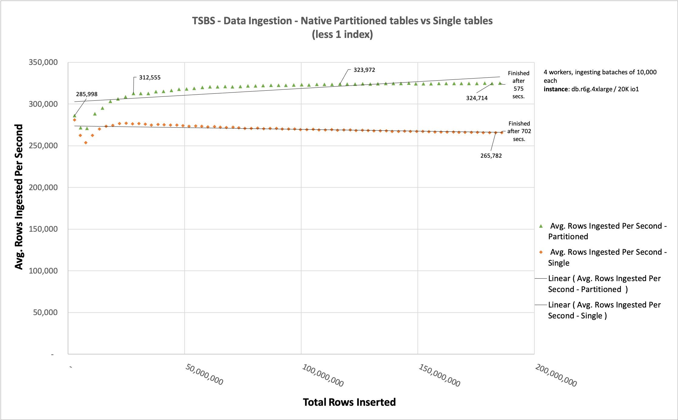
The data ingested is exactly the same. The only difference when comparing this chart with the previous one is the presence of those two indexes. Removing them reduced the difference between ingesting partitioned tables and single tables by 127 seconds, whereas previously that difference was 944 seconds.
When talking specifically about data ingestion, partitioning a table helps when data is being ingested because this strategy makes the individual index of each partition smaller.
Other ingestion examples: pgbench
The PostgreSQL community has a default and relatively easy-to-use benchmark tool called pgbench. When PostgreSQL 13 was released, a feature was introduced in pgbench that’s worth mentioning because we’re talking about partitions.
By default, the pgbench tool works in two modes: initialization mode and benchmarking mode. These modes are distinguished by one parameter: --initialize, or simply -i. You must initialize it the first time you’re benchmarking using pgbench. In other words, you create the tables, primary keys, foreign keys, and populate those objects. Starting with PostgreSQL 13, you can initialize your dataset in a partitioned manner. For that you must use the parameter --partitions=NUM.
The parameter says that you’re creating the pgbench_accounts table in a partitioned way, and NUM defines who many partitions you want to have. The default value is 0, which means the table isn’t partitioned.
Bearing in mind the PostgreSQL environment variables are still set, you can initialize your dataset in a partitioned manner by using the following command:
Note the way in which this partition is implemented. It uses the range partitioning method with eight partitions, where partition 1 accepts all values less than 1250001 and partition 8 accepts all values greater than 8750001.
This isn’t ideal, because if the table keeps growing (imagining a scenario where the partition key (aid) keeps receiving new values), partition 8 (pgbench_accounts_8) has many more values than other partitions. To prevent partition 8 from becoming overly skewed, partition 9 should be added before aid reaches 10,000,000.
Another approach for partitioning is, instead using the range method, to use the hash partition method. As the name suggests, the hash method relies in a hash function to distribute rows across a pre-determined number of partitions. That is particularly helpful when you’re partitioning by a primary key or any value that you know can be equally distributed and the access for these particular rows is pseudo-randomized. Although hash partitions keep all the partitions the same relative size to each other, they all grow as more values are added to the table. This reduces or even eliminates the performance advantages of range partitions.
pgbench introduced another parameter in PostgreSQL 13 called partition-method to allow for hash or range partitioning. By default, range partitioning is used, where each partition is used to handle a specific internal of the partition key. For example, partition 7 holds values that occur for the aid column between 7500001–8750001. Another partition range example is what we used during the tsbs benchmark tests in the previous section, in which each partition handles a particular range of timestamps.
To illustrate how a table partitioned by hash looks like, instead of running pgbench -s 100 -i --partitions=8 as we did earlier, we now specify that we want to initialize the benchmark using a hash method for our partitions. For that, we use the following command:
The partitioned table looks like the following:
With the hash method, instead of having a pre-determined range for the partition column (aid) defining which partition the row is, we have a modulus of 8 (the number of partitions) for the aid column. Then, depending on the remainder, a determined partition is chosen to store a particular row.
Combining partition methods: Sub-partitions
When talking specifically about time series data ingestion, you can combine range methods (to handle the timestamp columns, which defines which sub-partition the row should be). Then you can use the hash method for primary keys to ensure more evenly distributed and even smaller partitions.
The following code creates a table named readings and sub-partitioned tables:
The readings table uses a multi-hierarchical partitioned approach, first using the time column as a range to spread data across multiple partitions determined by specific intervals. We call that sub-partitioning. Below the readings table, two partitions are defined by using a range for the time column and one default partition. We have sub-partitions below each of those two partitions defined by range. In our example, we have three sub-partitions, partitioned using hash partitioning on the tags_id column. These partitions are leaf partitions, which store all the data. All other partitions above the bottom leaf partitions are empty. They’re used as a path to find the correct sub-partition (allowing faster access when reading it). We also create a default partition to catch all ranges outside the ranges that we defined as partitions.
Summary
In this post, we covered how to speed up data ingestion by taking advantage of the PostgreSQL native partition functionality that you can use with Amazon RDS for PostgreSQL or Amazon Aurora PostgreSQL-Compatible Edition. The idea of partitioning is that the database engine performs better by having smaller chunks of data to process when compared to processing a single, large table. This is true not only when you need to read the table, but also when you ingest new rows of data. Partitioned tables split larger datasets so the engine has better performance by using smaller chunks of data when compared to a single and large table.
We also discussed five distinct factors that contribute to data ingestion performance: table size, indexes, ingestion method, checkpoints, and Availability Zones.
Then we used benchmarks to demonstrate the performance improvement when ingesting 186,706,431 rows using partitioned tables in 820.360 seconds against non-partitioned tables in 1784.768 seconds (a decrease of 54% in ingestion time).
Finally, we compared the same data ingestion after removing one index from each table. The partitioned table ingested all 186,706,431 rows in 127 seconds, and non-partitioned table took 994 seconds, which demonstrates the impact of indexes on data ingestion.
We encourage you to try out this solution, and leave your feedbacks, thoughts and ideas in the comments.
About the Author
 Vinícius A. B. Schmidt is a Database Engineer specialized in PostgreSQL at AWS. He is passionate about databases, security and mission critical systems. Prior to joining AWS, Vini was both a PostgreSQL consultant and instructor working with customers in public and private sectors in many continents. He has been designing, implementing and supporting solutions based on open-source technology since 1999.
 Andy Katz is a Senior Product Manager at Amazon Web Services. Since 2016, Andy has helped AWS customers with relational databases, machine learning, and serverless workflows.